Introduction to different ways of representing 3-Dimensional information (3D). 

Discrete Representation

As a common trend in the process of mimicking reality, we have reduced the amount of data captured in order to gain speed, especially for real time simulations such as games. How much granularity do we need in able to display an apple for example? The answer is enough for our purpose.

Vertices

Vertices are the smallest unit used in graphics engines. They have applications in both 2D and 3D simulation and they basically represent a point.

struct Vertex {
    float v[3];
}

Vertex is basically a point in 3D space. So we store an array of three floats to hold that information.

Polygons

Polygons are made up of vertices. The most common polygon used in graphics engines is the triangle which is composed of three vertices. Followed by Quadrilaterals with four vertices and on and on. The reason for triangles is many, but one of them is the triad partitioning which many graphic cards are optimized for.

struct PolygonTriangle{
    int indexes[3];
}

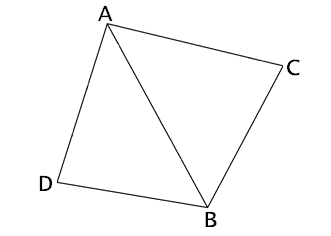
A polygon triangle, simply know as a triangle will hold three indexes which will prove to be useful in building a mesh without duplicating vertices. Adjacent triangles share one or more vertices.

As you can see in the picture above, both triangles share vertices: A and B.

We would need only four vertices and three indexes for each of the triangles versus of six indices, if we stored actual vertices in every triangle.

Mesh

All these polygons are compiled into a mesh; synonymous to an object. These have their local vector spaces in order to keep track of the vertices and polygons they contain.

struct Mesh{
    Vertex vertices[VERTEX_COUNT];
    PolygonTriangle polygontriangles[POLYGON_COUNT];
}

A mesh will typically have an array of vertices and an array of polygon triangles whose indices point into the vertices array. As explained above this is highly optimal during the different rendering pipeline stages.

RASTERIZATION DEMO 

Continuous Representations

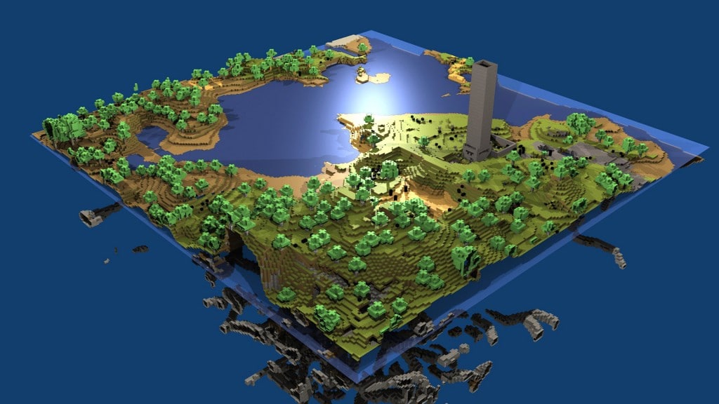
Continuous representation research has been embarrassing compared to its discrete counterpart. Although efforts are started to show some good progress. Minecraft is a good example although it is an extremely representation and it doesn’t even render the voxels as volumes but converts them to triangles pre graphics card submission.

Another great example of voxel rendering that actually renders volumes is Atomontage Engine.

 I must first differentiate and define Continuous representations. We have the actual equations that yield rendering data per rendering frame and low resolution 3D grids as used in such products as Minecraft and in Medical Imaging.

Voxel Representation (Volumetric Pixel)

This representation of 3D is akin to 2D Bitmaps. Where every 3D coordinate in the world is either occupied or not. This can quickly fill up the computer’s memory with fairly mediocre results.  Of course the higher the resolution the more precise the model; cue Medical Imaging.

 A naive representation of volumetric 3D worlds would begin as…

struct Block {
     Texture image; // if textures are needed
     int r, g, b, a; 
     //...
}

struct World{
    Block blocks[WORL_SIZE_X][WORLD_SIZE_Y][WORLD_SIZE_Z];
}

The world would be broken down into blocks (the smaller the blocks, the higher the definition). Each block would contain certain properties that would indicate to the renderer how to draw it. Taking into account all the visual properties like specular, shading, color, opacity etc.

Parametric Functions

These functions are the true “continuous” representation as they would output results for any given precision. They range from Bezier curves to multi-variable equations that would define a surface’s property between given points. I must confess that they are hard to use especially when the limits are far between each other. Graphics researches have found solutions by keeping their boundaries low and using a lot of them together, this technique is known as Bezier Patches.

So what is a Bezier curve?

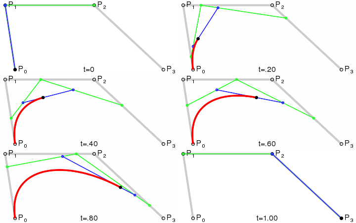
As you can see, Pn where n:0…3, are all control points. Between these points, the Bezier equation will fill a curve. The more control points you add, the more the curve can be influenced. For four points, it’s known as the Cubic Bezier Curve. The mathematical drawing is as follows:

Each line is defined as its initial point plus its normalized slope which is multiplied by the scalar ‘t’ which goes form 0…1. This will create a line between points P0 and P1.

       P0 + (P1-P0)t where  0 <= t <= 1

Simlarly for points P1 to P2 and P2 to P3.

      P1 + (P2-P1)t where  0 <= t <= 1

      P2 + (P3-P2)t where  0 <= t <= 1

 Now once, these lines are defined we draw a line between them as they have the variable ‘t’ in common. This will yield a segment where a line is formed by a linearly moving point controlled by the parameter ‘t’.

What’s next

This has been a quick rundown of the current state of data representation in 3D Rasterization Architectures. Future posts will delve into texture and shading as well as a more thorough discussion of the light equation in these matters (get your math and physics brains out!).